Two ways we tried to stop overestimating residual risk

This is a shorter companion post for “Accurate and Low-Cost Residual Risk Assessment via Sampled Profiling and Structure-Aware Coverage Amplification” (ASE ‘26), which I wrote with Seongmin Lee, Marcel Böhme, and Miryung Kim. I want to connect it to Seongmin and Marcel’s earlier paper, “Dependency-aware Residual Risk Analysis” (ICSE ‘26), and instead of just restating our three RQs and their results, I want to write them out as the questions we were actually asking, along with what we expected going in.

Okay, but what even is residual risk?

Before any of that, it’s worth being concrete about the term itself, since it’s doing a lot of work in both papers. Say you’re fuzzing a program: throwing generated inputs at it and watching for crashes. At some point, the fuzzer stops finding new bugs for a while. Does that mean the program is clean, or does it just mean you haven’t gotten unlucky yet?

Residual risk is the answer to that question stated as a probability: given everything the fuzzer has found so far, how likely is it that the next test input triggers a bug nobody’s seen yet? If that number is high, you should keep fuzzing. If it’s low, you’re probably wasting compute by continuing, and that budget would do more good on a different target. The whole point of estimating it is to turn “should I stop fuzzing this target” from a guess into a number you can actually threshold on.

The catch is that you can’t compute this directly, because you’d need to know the true, unknown distribution of bugs still hiding in the program. So both papers below are really about the same narrower question: given only what a fuzzing campaign has observed so far, how do you get the best possible estimate of that unknown risk?

Why we were both staring at the same problem

Seongmin and Marcel’s ICSE ‘26 paper and our ASE ‘26 paper both go after the same weak spot: the Good-Turing estimator (GoTu) that prior residual risk work relies on tends to overestimate risk, so testers keep fuzzing long after they should’ve stopped. But the two papers go after that overestimation from two different directions, and it’s worth naming exactly what each one is doing.

In the ICSE ‘26 paper, Seongmin and Marcel’s argument is that the overestimation is structural. GoTu treats coverage elements as if they’re independent of each other, when really some blocks are only reachable once other blocks have already been hit. Their fix doesn’t touch program analysis at all. Instead, they infer the dependency structure statistically, just from how coverage elements co-occur across sampled executions, using Ma and Chao’s sample coverage estimator. That alone gets their median error down to about a fifth of GoTu’s.

In our ASE ‘26 paper, we went after a different piece of the same problem. Our argument is that the overestimation is partly observational: coverage instrumentation is accurate, but it’s slow (60 to 70% slower), and that slowness throttles how many executions you can even run in the first place. So we asked a blunter question:

Can we get rid of coverage instrumentation altogether?

Our answer was to swap it for hardware instruction-pointer sampling, which is much cheaper but also much sparser, and then recover the coverage we lost using must-execute analysis: a static control-flow argument that says “if we observed this block executing, these other blocks must have executed too.” Here’s what that looks like on a small example program:

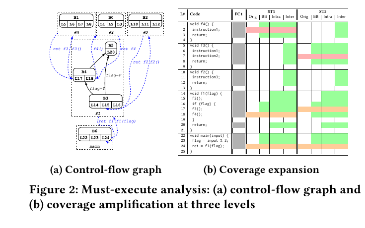
Reading these two papers back to back, they stop looking like two separate fixes and start looking like two halves of the same argument. One of us is saying the data you’re measuring is misleading you even when it’s complete. The other is saying measuring completely is the thing slowing you down in the first place.

RQ1: is the estimate actually any good?

The question we were asking here was simple: if we throw away most of our coverage data and only keep sparse, sampled snapshots, how far off does our risk estimate end up from the real thing?

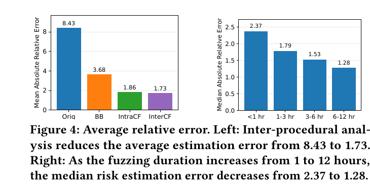
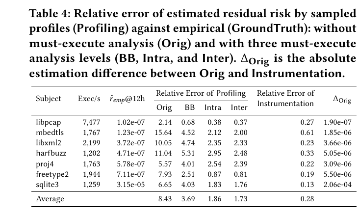
Our hypothesis was that must-execute analysis should close most of that gap, because it’s recovering coverage we know must have happened, not guessing. What we found matched that: without any must-execute analysis at all, our estimate is way off, close to an order of magnitude off from the ground truth. Layering on inter-procedural must-execute analysis brings that error way down, and it keeps getting better the longer the campaign runs. You can see the shape of that in the paper’s own numbers:

And here’s the full per-subject breakdown, which is worth a look if you want to see how this plays out differently across real codebases like sqlite3, mbedtls, and libxml2:

RQ2: does dropping instrumentation actually buy us anything?

This one is more of a sanity check than a leap of faith: if we’re giving up complete coverage data, we’d better be getting real throughput out of it. Our hypothesis was that removing instrumentation overhead should let the fuzzer run meaningfully faster, and that faster execution should translate into finding more bugs in the same amount of wall-clock time. That’s what we saw. We were noticeably faster than instrumentation-based fuzzing, and that speed showed up directly as more bugs found within the same time budget.

RQ3: does any of this actually help you stop sooner?

This is the question that actually matters if you’re the one running the fuzzer: does the estimate, even if slightly noisier, let you make a good stopping decision faster than waiting on full instrumentation? Our hypothesis was that the throughput gain from RQ2 should outweigh the small accuracy cost from RQ1, at least at low sampling frequencies. We found that in most of our configurations, yes, we hit the stopping threshold sooner with profiler-based sampling than with instrumentation, and the advantage gets bigger the stricter the threshold you’re asking for.

Where this leaves an open question

Here’s the thing neither paper answers on its own. The dependency-aware estimator’s overhead is almost entirely in analysis, not in per-execution instrumentation, so it’s cheap to run alongside a fast fuzzer. That makes me want to ask: if we ran dependency-aware DP estimation directly on top of profiler-sampled, must-execute-amplified coverage, would the gains from both papers actually stack? Or are they both just recovering the same slack in GoTu from different angles, in which case stacking them wouldn’t buy us much once we’d already applied one? That’s the natural next experiment, and as far as I know nobody’s run it yet.